As mentioned in our blog post about OData support in Mendix, OData is also useful if you want to access data in your applications from R or RStudio. In this blog post, I’ll show you how to do this. I’ll also give some simple examples of how to use R aimed at people who are unfamiliar with it.
What is R?
R is a very popular Open Source Statistical Analysis programming language used by many data scientists. You can download a free, open source version, but you’ll also find R support in many commercial tools, including Microsoft Revolution R, Tibco Spitfire, Pivotal, Oracle, and Tableau. What’s interesting about R is that there are a large number of libraries that you can use. Libraries range from data manipulation algorithms, to graphing, to reporting, to machine learning.
Loading OData into R
To retrieve OData into R we’re going to use two packages: httr and XML. The first package enables you to read data from the web, the second can be used to parse XML documents.
With a small function using these packages, you can fetch a OData resource and turn it into R data.
dataset <- getODataResource(<url of the odata resource>,<username>,<password>)Before we start we need to specify the libraries we need.
library('httr')
library('XML')
library('dplyr')
library('lubridate')
The function getODataResource first reads the OData resource and parses the returned XML document using the Httr package. Next, it determines the names of the attributes, gets the values, and builds a data frame containing the values.
getODataResource <- function(resourcePath,domain,usr,pwd){

  url <- paste(domain, resourcePath,sep="")
  # get the OData resource
  response <- GET(url,authenticate(usr,pwd))

  # parse xml docucument
  responseContent <- content(response,type="text/xml")

  # determine the names of the attributes
  xmlNames <- xpathSApply(responseContent,
      '//ns:entry[1]//m:properties[1]/d:*',xmlName,
      namespaces = c(ns = "https://www.w3.org/2005/Atom",
        m="https://schemas.microsoft.com/ado/2007/08/dataservices/metadata",
        d="https://schemas.microsoft.com/ado/2007/08/dataservices"))

  # determine all attribute values
  properties <- xpathSApply(responseContent,'//m:properties/d:*',xmlValue)

  # cast the attributes values into a data frame
  propertiesDF <-
      as.data.frame(matrix(properties,ncol=length(xmlNames),byrow=TRUE))

  # set the column names
  names(propertiesDF) <- xmlNames
  return(propertiesDF)
}
This is the basic functionality that you need to retrieve Mendix OData resources into R. In its current form, it doesn’t handle nested data, so for example, Orders with order lines nested in the orders. It also doesn’t use the datatype info that is included in the OData resource. Instead, we’ll use some R expressions to specify the data types manually, as illustrated below.
Example use case
The example Mendix application has resources for orders, customers and addresses. We’ll create an overview of the number of orders per city in R.
First, we’ll define how to connect to the OData resources in our Mendix application.
domain <- "https://localhost:8080/"
username <- "demo_reporter"
password <- "goSfcsDj00"[/bash]

The following will load all the objects in the customers and address entities into R data frames.

[bash]customers <- getODataResource("odata/Orders/Customers()",domain,username,password)
addresses <-  getODataResource("odata/Orders/Address()",domain,username,password)
For orders we’re just interested in the orders created since january 1st 2014. We could filter on order date in R, but specifying it on the OData resource url avoids the overhead of querying them from your Mendix database, and transporting all the data from the Mendix runtime to R.
orders <- getODataResource(
  "odata/Orders/Orders()/?$filter=OrderDate%20gt%20datetimeoffset'2014-01-01T00:00:00z'"
  ,domain,username,password)
The data frames contain all the Mendix objects, retrieved through OData resources. The first five records of orders look like this:
orders[1:5,c("OrderNumber","Order_Customer","OrderDate")]## OrderNumber Order_Customer OrderDate
## 1 1 2533274790395905 2015-01-18T10:32:00.000Z
## 2 2 2533274790395906 2014-01-30T07:01:00.000Z
## 3 3 2533274790395907 2014-04-16T13:15:00.000Z
## 4 4 2533274790395908 2014-09-19T07:52:00.000Z
## 5 5 2533274790395909 2015-01-14T07:28:00.000ZNow that we have the data, we need to make sure we use the correct datatypes. Mendix IDs are implemented using longs in Mendix. In R, you can use doubles.
customers$DateOfBirth <- ymd_hms(customers$DateOfBirth)
customers$ID <- as.double(customers$ID)
customers$Billing_Address <- as.double(customers$Billing_Address)
customers$Delivery_Address <- as.double(customers$Delivery_Address)

addresses$ID <- as.double(addresses$ID)

orders$ID <- as.double(orders$ID)
orders$Order_Customer <- as.double(orders$Order_Customer)
# for easy access, create separate columns with date and date time
orders$OrderDateTime <- ymd_hms(orders$OrderDate)
orders$OrderDate <- ymd(format(ymd_hms(orders$OrderDate),"%Y-%m-%d"))
Next we’ll use the dplyr library to manipulate the data received. Dplyr enables you to filter data, add new columns, select certain columns, and order the rows, very much what you would do with SQL in a regular database.
The following dplyr expression joins the customers, addresses, and orders data frames.
customerOrders <- customers %>%
  rename(CustomerID=ID) %>%
  left_join(addresses, by=c("Delivery_Address"="ID")) %>%
  select(CustomerID,Firstname,Lastname,City,Country) %>%
  left_join(orders, by=c("CustomerID"="Order_Customer")) %>%
  select(Firstname,Lastname,City,Country,OrderNumber)
The first rows of this data frame look like this:
customerOrders[1:5,]## Firstname Lastname City Country OrderNumber
## 1 Ivan Freeman New Orleans US 1
## 2 Ivan Freeman New Orleans US 499
## 3 Anthony Robinson Brighton US 2
## 4 Anthony Robinson Brighton US 500
## 5 Kaden Griffith Bridgeport US 3Now we can count the number of orders per city as follows:
cityOrderCount <- customerOrders %>%
  group_by(City) %>%
  summarize(OrderCount = n()) %>%
  arrange(desc(OrderCount))
The result:
cityOrderCount[1:5,]## Source: local data frame [5 x 2]
##
## City OrderCount
## 1 New York 28
## 2 Philadelphia 16
## 3 Chicago 15
## 4 Miami 12
## 5 Baltimore 10Creating graphs
The following example uses ggplot2 to create graphs. You can also use other libraries for graphing, but ggplot2 is one of the more popular.
We’ll start with a simple bart chart plotting the number of orders per month.
library('ggplot2')

# Determine first day of month for every order, count number of orders per month

orderCount <- orders %>%
  # Determine date of first day of the month, so ggplot understands it's a date
  mutate(OrderMonth = ymd(format(OrderDate,"%Y-%m-01"))) %>%
  group_by(OrderMonth) %>%
  summarize(noOfOrders = n())

# generate barchart to display number of orders per month

ggplot() +
  geom_bar(data=orderCount,aes(x=OrderMonth,y=noOfOrders), stat="identity") +
  xlab("Month") +
  ylab("Number of orders") +
  ggtitle("Orders per month")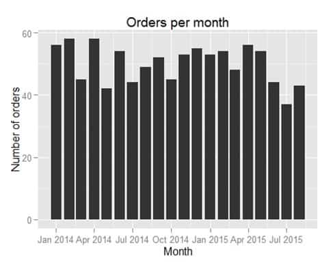
Next we’re interested in seeing when orders are placed during the week. First, we need the dataset, containing day of week and hour of day for every order.
ordersPerWeekHour <- orders %>%
  mutate(DayOfWeek = wday(OrderDate)) %>%
  mutate(HourOfDay = hour(OrderDateTime)) %>%
  group_by(DayOfWeek,HourOfDay) %>%
  summarize(noOfOrders = n())
Now for the actual graph, we can use tile plane to show the number of orders for every hour of every day. We put the day on the x-axis, the hour on the y-axis, and use number of orders to determine the color displayed.
ggplot(ordersPerWeekHour, aes(x=DayOfWeek,y=HourOfDay))+
  geom_tile(aes(fill=noOfOrders)) +
  scale_fill_gradient(low="green", high="red") +
  scale_x_continuous(breaks=1:7,labels=c("Sun","Mon","Tues","Wed","Thurs","Fri","Sat")) +
  scale_y_continuous(breaks=0:24) +
  labs(x="Day", y="Hour")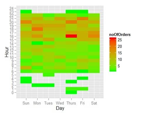
You can now easily see that most of the orders are placed between 16:00 and 22:00, evenly divided across all days of the week.
Generate reports using R
R has some interesting reporting facilities. Using Rmarkdown, you can generate HTML, Word, PDF or even slides straight from an R report.
This whole blogpost was actually written using rmarkdown, generating an MS-Word document. To update the Word document with the latest data from my Mendix application, I just have to rerun the rmarkdown script.
The easiest way to work with Rmarkdown is to use the built-in facilities of RStudio. Alternatively, you can generate an Rmarkdown report without RStudio with some R code:
library(knitr) # required for knitting from rmd to md
require(rmarkdown) # required for md to html
setwd('<location of your rmarkdown file>')
render("<name of the rmarkdown script>", "all")
Conclusion
The OData feature in Mendix opens up a lot of possibilities for Mendix users. R is a powerful tool for statistical analysis and data reporting. Using OData Mendix user can now easily benefit from all these facilities.